Calibration
of a TOF powder diffractometer
In this tutorial, data collected on the SNS instrument POWGEN, are used. The calibration process will use the fitted positions of all visible peaks in a pattern of NIST SRM 660b La11B6 (a=4.15689Å) obtained in a multiple single peak fit. The positions will be compared to those expected from the known lattice parameters to establish the diffractometer constants (difC, difA, difB and Zero) used for calculating TOF peak positions from d-spacings. For the second part of this tutorial, the suite of peaks will be extended to include every visible peak in the pattern and the peak fitting will include the various profile coefficients thus fully describing the instrument contribution to the peak profiles. Note that menu entries and user input are shown in bold face below as Help/About GSAS-II, which lists first the name of the menu (here Help) and second the name of the entry in the menu (here About GSAS-II).
If you have not done so already, start GSAS-II.
Part I. Determine the diffractometer constants
Step 1: Read in the data file
Use the Import/Powder data/from GSAS powder data file menu item to read the data file into the current GSAS-II project.
A file selection dialog will be shown; its appearance will
depend on your OS. Change the search directory to TOF
Calibration/data and then select the file PG3_17541.gsa
and press Open. A window will
appear “Is this the file you want?”. Press Yes. The file selection dialog will reappear; select the PGHR_60-2015A.prm file. It
contains the POWGEN instrument parameters provided along with the data; this
file is in the old GSAS iparm file format and does not include all the
instrument parameters used by GSAS-II. This is what we will be improving in
this tutorial.
At this point the data tree window will have several entries and the powder pattern will appear. Next, select the Limits item in the GSASII Data tree under PWDR PG3_17541.gsa Bank 1 and set the lower limit to be at the end of the pattern (easily done by dragging the green dashed line to below the end of the pattern; it will snap back to the 1st point).

Step 2: Select peaks
Under the PWDR PG3_17541.gsa Bank 1 GSASII Data tree item find the Peak List entry; it will be empty. Select the menu item Peak Fitting/Auto search to populate the Peak List. This will select almost every peak in the pattern (I got 66 peaks).
However, it can fail by selecting a peak multiple times if the data is too noisy. You should check through the list and eliminate any close duplicates (in this instance there didn’t appear to be any). A peak can be eliminated by placing the cursor on the vertical blue line and pressing the right mouse button; the line should vanish and the entry in the table deleted. Notice that the position for the highest 2 TOF peaks are misplaced. You can shift them by placing the cursor on the blue line and with the left mouse button down, drag each line to match its peak top (zooming in before can help). If you want you can add more of the unpicked lines to the list (I didn’t). To do this (zooming in helps) place the cursor on a data point at the top of a peak and press the left mouse button. It is easiest to proceed from right to left so the tool tip stays out of the way as you work. For any of these operations the zoom buttons at the bottom left of the plot window must be turned off.
Step 3: Fit peaks
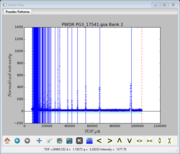
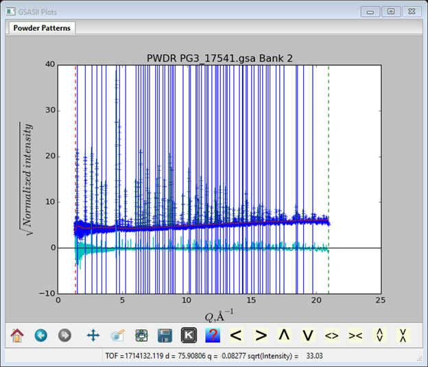
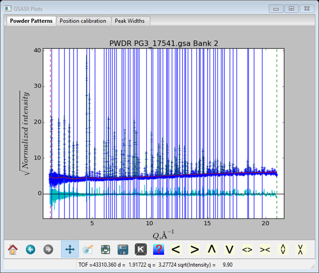
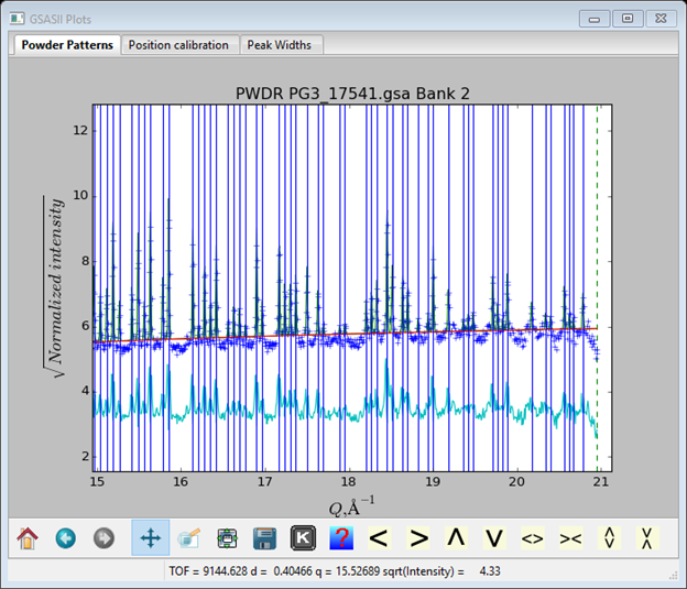
To do the initial fit to the peaks, select the Peak Fitting/Peakfit menu item in the data window. GSAS-II will ask for a project name before continuing, enter a name (I chose calibrate). The project file (calibrate.gpx) will be written into your local directory selected in the File Dialog; then the refinement will proceed. The resulting plot will look like (I keyed ‘s’ and ‘q’ on the plot to get a sqrt(I) vs q plot which spread out the peaks a bit better than a I vs TOF plot).

The fit to the background can be improved by adding more terms; I set the number of chebyschev terms to 6. The peak positions should also be refined; to set them go back to the Peak List data window, select one of the items under the 1st refine column, select the “refine” box (the column will turn blue), then press y. All the position refine boxes will be checked. Then repeat the Peak Fitting/Peakfit menu item; a new plot will appear with a better fit.
Step 4: Setup for calibration
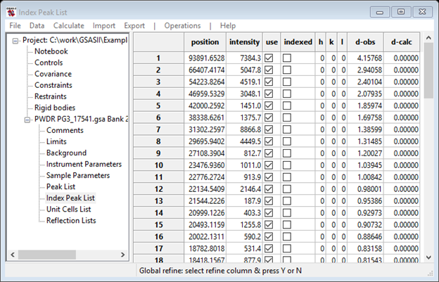
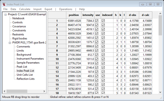
Now that we have a reasonably well fit set of peak positions, we next need to index them with respect to the lattice parameters of the standard. Select the Index Peak List entry in the GSAS-II Data tree, an empty data window will appear. Populate it by selecting Operations/Load/Reload menu item. The data table will show the positions & intensities along with 000 for hkl for each one.
Next, select the Unit Cells List from the GSAS-II Data tree. A new window will appear. Change Bravais lattice to Pm3m, select P m 3 m for the Space group and enter the lattice parameter (4.15689) in the Unit cell: a = box (Press Enter to set the value). The window should look like
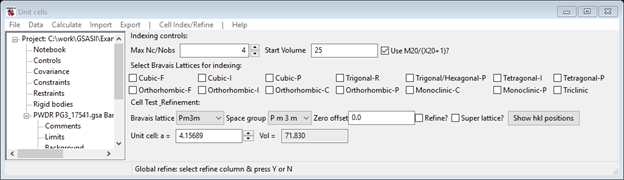
Press the Show hkl positions button, the plot should show a suite of red dashed vertical lines giving all the allowed reflection positions which should closely match the blue peak position lines.

The Index Peak List window now shows hkl values for each entry
The calibration set up is now complete.
Step 5: Calibration of diffractometer constants
As we now have a set of reflection positions each properly indexed so that the d-spacings are known, we can now determine the diffractometer coefficients (C, A, B and Z) that give TOF from d-spacing according to
![]()
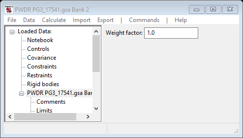
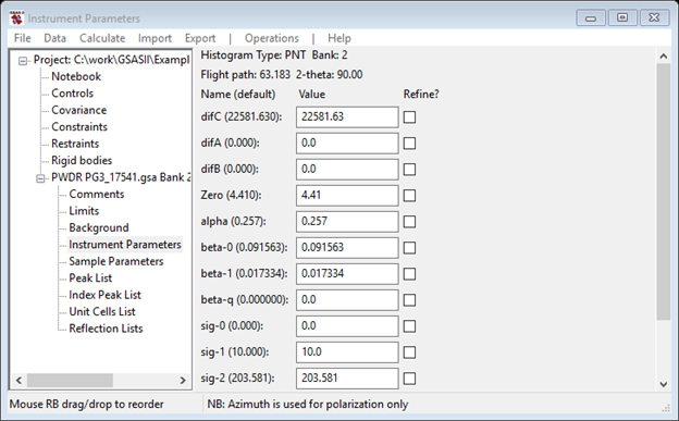
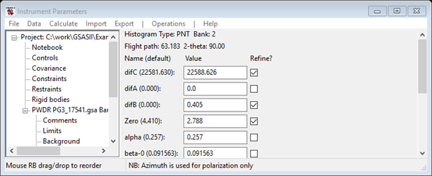
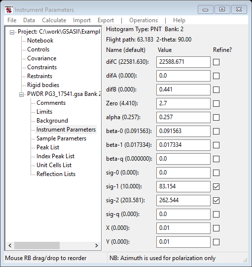
Select Instrument Parameters from the GSAS-II Data tree. The data window will show
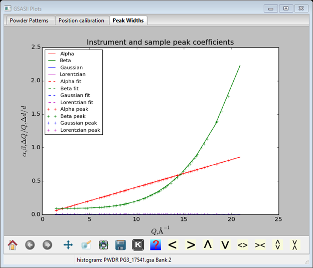
And the plot will show the corresponding function curves
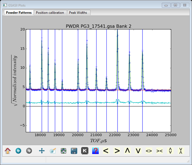
Although a previous calibration gave values for difA and Zero, we will start fresh; set them both to zero. Select the difC Refine? box and do Operations/Calibrate; the plot will show the result of the calibration
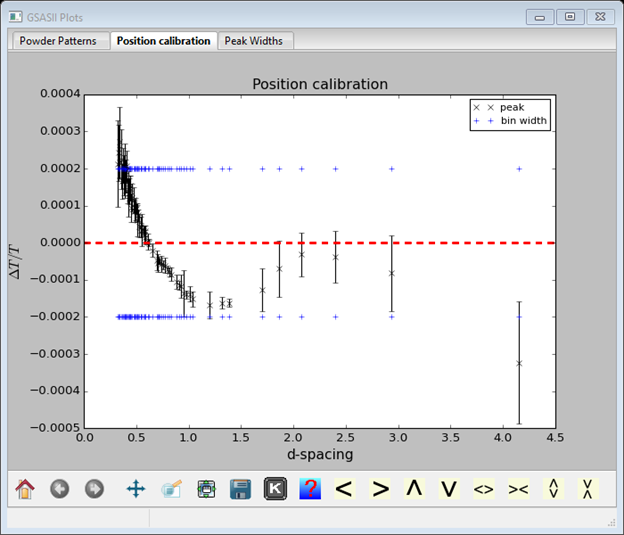
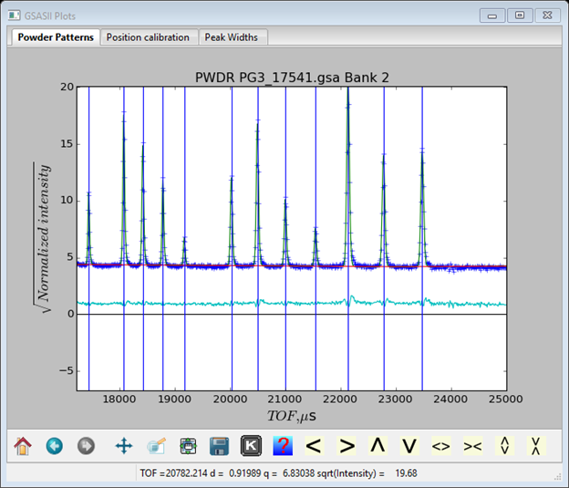
If you have any very bad data points (far outside the blue bands), you should remove them. Use the mouse cursor to determine their position so you can find it in the Index Peak List. Select that data item from the tree. Uncheck the use box for it. Go back to Instrument Parameters and repeat Operations/Calibrate; the plot will look a lot better.
What is shown is the discrepancy between observed and calculated position divided by the position (ΔT/T) vs d-spacing. The error bars reflect the uncertainty in the fitted peak positions. The red dashed line is obviously zero discrepancy and the blue dashed lines represent the width of a data bin above and below zero (e.g. 2 bins from one blue line to the other) to give you a sense of how significant the discrepancies are. One can improve the fit by including the difB and ZERO parameters; select them and repeat Operations/Calibrate. The fit is much improved.
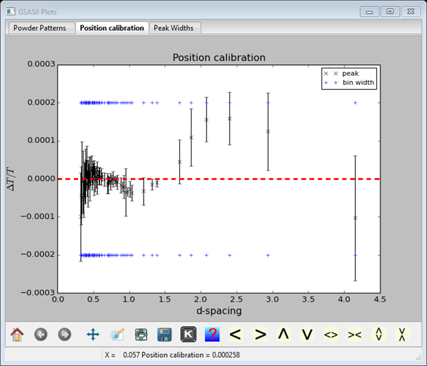
One might get some improvement by refining DifA. I got the following
new parameters
The fitted values are clearly about one TOF bin of zero or less.

As these values have now been established, uncheck all their refinement boxes. This ends the first part of this tutorial exercise; you may save the project if you wish, select File/Save project from the GSAS-II data tree window. Notice that we did not establish values for the instrument profile coefficients (alpha, beta & sig terms). These will be established in the second part of the tutorial.
Part II. Determine the instrument profile coefficients
To best establish the profile coefficients one must have the best model for the fitting. In this case we will change the background function to something more flexible than the 6 term chebyschev function used above and add all visible peaks beyond those found by the automatic procedure used above.
Step 1. Change background
Select the Background tree item; you should see

From the Background function pulldown, select log interpolate and set the No. coeff. to 10. This will select 10 fixed position points across the pattern between the limits located in constant log(TOF) steps; this puts more points at the short TOF end of the pattern where the background is changing most rapidly. Return to Peak List and do Peak Fitting/Peakfit; this should give a better fit to the background.
Step 2. Add more peaks to be fitted
Now zoom in on the right hand end of the pattern and select every unmarked peak you can see. Be sure the zoom button is off and you can use the < > buttons to shift the pattern left or right. It is essential to include as many peaks as possible because including them forces the background to its “true” level and thus giving each peak its true shape. The high Q end of my pattern looked like

When I was done; I had 130 peaks. Do Peak fitting/Peakfit; all peaks should fit in a few seconds and the background line should drop a bit.
I’ve dragged the difference curve up so you can see it. Notice that it is mostly from position errors; so set the refine boxes for position (i.e pick a box, pick the refine column heading & press y). Repeat Peak Fitting/Peakfit; the fit will improve. On the console listing before the peak listing the residuals are shown; Rwp ~13%
You might want to save the project at this point; do File/Save project from the main GSAS-II data tree window.
Step 3. Refine profile coefficients
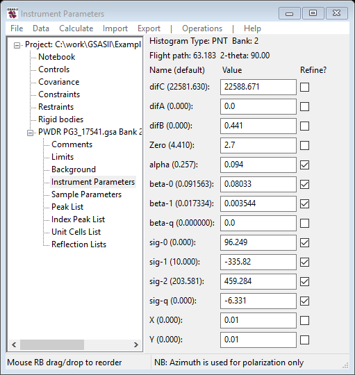
In this step you will be selecting some profile coefficients (alpha to sig-q) for refinement, doing peak fits and hopefully improving the fit to the profile. Occasionally the refinement will diverge or fail; use the Peak fitting/Undo command immediately to recover. The Background, Instrument Parameters and Peak List values will all be restored. Select Instrument Parameters from the GSAS-II data tree; the data window will show

You should realize that alpha largely affects the sharpness of the leading TOF edge of each peak; larger values mean sharper front edges. Beta terms affect the trailing TOF edge in the same way. Sig terms affect the Gaussian shape component of the peak profiles; larger values result in broader peaks. The coefficients describe the alpha, beta and sig values as follows:
![]()
![]()
![]()
The refinable coefficients are: alpha (α0),
beta-0 (![]() ), beta-1 (
), beta-1 (![]() ), beta-q (
), beta-q (![]() ), sig-0 (
), sig-0 (![]() ), sig-1 (
), sig-1 (![]() ), sig-2 (
), sig-2 (![]() ) and sig-q (
) and sig-q (![]() ). Some of the values given
above are probably not appropriate; looking at the difference curve it appears
that the peak width is most in error. Refine sig-1 and sig-2.
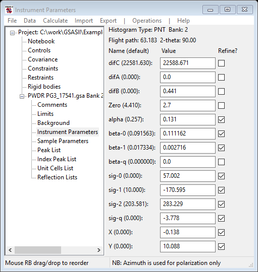
Remember to go back to Peak List to do the fitting. My Rwp improved to 7.17% and the new coefficients looked like
). Some of the values given
above are probably not appropriate; looking at the difference curve it appears
that the peak width is most in error. Refine sig-1 and sig-2.
Remember to go back to Peak List to do the fitting. My Rwp improved to 7.17% and the new coefficients looked like
After adding sig-0 and sig-q to the refinement, my residual improved slightly to Rwp=6.05%. A zoom view of some peaks around TOF~20000µs

Suggests that the beta terms are too large, i.e. the trailing edges are calculating too sharp compared to the data. In two steps first add beta-0 to the refinement and then second add beta-1. The two refinements improve the fit (Rwp=5.6% after the 1st step and Rwp=5.4% after the 2nd). The resulting coefficients are

And the fit in the above region is now much better.
The principal errors now seem to be on the front edge of the peaks. After adding alpha to the refinement, I got Rwp=4.45% and the difference curve is almost flat.
The coefficients are
As this represents a very good fit to the profile, it would be useful to save the project (do File/Save project from the main GSAS-II data tree menu) and make a new instrument file (do Operations/Save profile from the Instrument Parameters menu; you can overwrite the existing one). I did try to refine beta-q; that gave a failed refinement. However, the material used for the calibration (SRM 660b La10B6) does have some sample broadening. As this almost always shows up as a Lorentzian contribution to the peak profiles one can accommodate it by refining X and Y. After refining them I get a substantial improvement Rwp=3.24% and there are considerable changes in the other coefficients because they no longer have to compensate for the missing Lorentzian component. Their values then represent the instrument contribution to the profile.
The profile fit is almost perfect
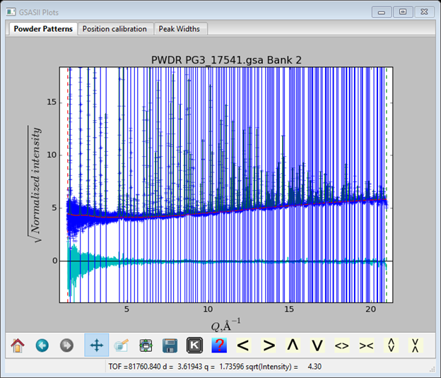
I’ve switched back to a q plot and positioned the difference curve to be about zero.
Step 4. Check diffractometer constants
Since these calibration fits for profile coefficients varied the peak positions, a final check on the diffractometer constants is needed. To do this, the new peak positions need to be loaded into the Index Peak List (do Operations/Load/Reload in that menu). Notice that the Index peaks are no longer indexed. In Unit Cells List, press the Show hkl positions button; this will index the lines. The go to Instrument Parameters and uncheck all the profile coefficient Refine? boxes; then check all the coefficients (difC, difB, difA & Zero). Do Operations/Calibrate. The agreement shows some deviations at very short d-spacing that weren’t evident in the initial calibration.
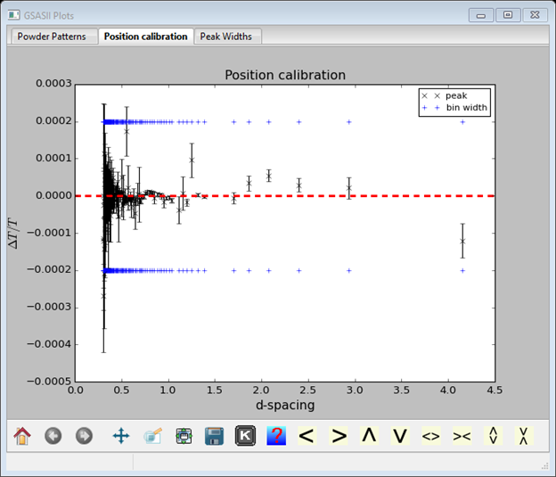
The fit now is better apart from a few stragglers at low d-spacings. These are very weak peaks whose position was poorly determined. Almost all the rest are within a 1TOF bin width around zero. Save the project (File/Save project in the main GSAS-II data tree menu).
Step 5. Make instrument parameter file
We now have a fully calibrated instrument with diffractometer coefficients and profile coefficients. Uncheck all refinement boxes and set X and Y back to zero. You should have

This removes from the instrument parameters any sample broadening effects and thus the remaining parameters are only dependent on the instrument. To make an instrument parameter file do Operations/Save profile; choose a suitable name expressing the particular instrument configuration used in collecting the calibration data. I named it POWGEN_1066.instprm (with the default extension) to reflect the wavelength band used to collect it on POWGEN. This completes this tutorial.